Welcome to the very beginning. This is the first project in a 6-step series that teaches mechanistic interpretability from "nothing" to "you can read research papers." If you've never trained a neural network in your life, start here.
Each step is structured as a notebook: a written walkthrough up top, then runnable Python code cells further down. You read, you run, you read more.
The goal of this project is to do the single most foundational move in interpretability: train a tiny model, then look directly at its weights and see that they mean something a human can recognise.
Specifically:
- We'll train logistic regression on MNIST (a famous dataset of 70,000 hand-drawn digits, used by everyone learning ML).
- We'll look at the model's weight matrix and see that each row is a fuzzy template of a digit.
- We'll then train a slightly bigger model (1 hidden layer) and look at its weights - they'll be messier and harder to interpret, which is a teaser for project 1 (superposition).
That single move - train, look, find something - is what every subsequent step in this series elaborates on.
By the end you'll have:
- Trained your first neural network.
- Visualised what it learnt by reshaping a weight matrix into images.
- Built the mental habit that "weights are not random - they have meaning, you can just look."
What is mechanistic interpretability?
When you train a neural network you get back a model defined by millions (or billions) of numbers - its weights. Nobody hand-designed those numbers. Gradient descent did (gradient descent = the training algorithm: nudge every weight a tiny step in the direction that reduces the model's error, repeat thousands of times). So they look, on first inspection, like noise.
Mech interp is the project of opening that "noise" up and discovering that, actually, the weights are doing something specific and understandable. The dream is a sort of "decompiler" for neural networks.
This first step is the simplest possible demonstration that opening the model up is worth doing. We train a tiny model, look at its weights, and see that they encode something a human can recognise.
If that move feels too obvious or too easy - good. The point is that all of mech interp is variations on this move, just applied to messier models with more sophisticated tools. Everything else in the curriculum complicates this picture.
The experiment in plain English
There are two experiments in this notebook, back-to-back.
Experiment A: logistic regression as template matching
Train the simplest possible model on MNIST:
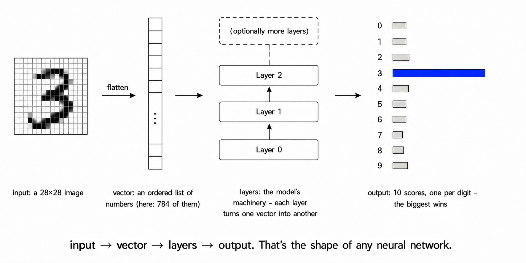
- Input: a 784-dim vector (flattened 28×28 image).
- Model: a single linear layer with 10 outputs. Total weights:
Wof shape(10, 784), plus a 10-dim bias. - Output: the model picks the class whose score is highest.
- Training: 5 epochs of Adam with mini-batches of 256 (~1,170 steps/epoch). Gets to ~92% test accuracy. Far from state-of-the-art, fine for our purposes.
After training, take the weight matrix W of shape (10, 784). Each row is a 784-dim vector - one per digit class. Reshape each row to 28×28 and plot it as a heatmap.
The picture below shows the trick in three stages: grab one row of W (it's just a long list of 784 numbers), reshape it into a 28×28 grid, then look at it. The "3" row, reshaped, looks like a fuzzy 3.
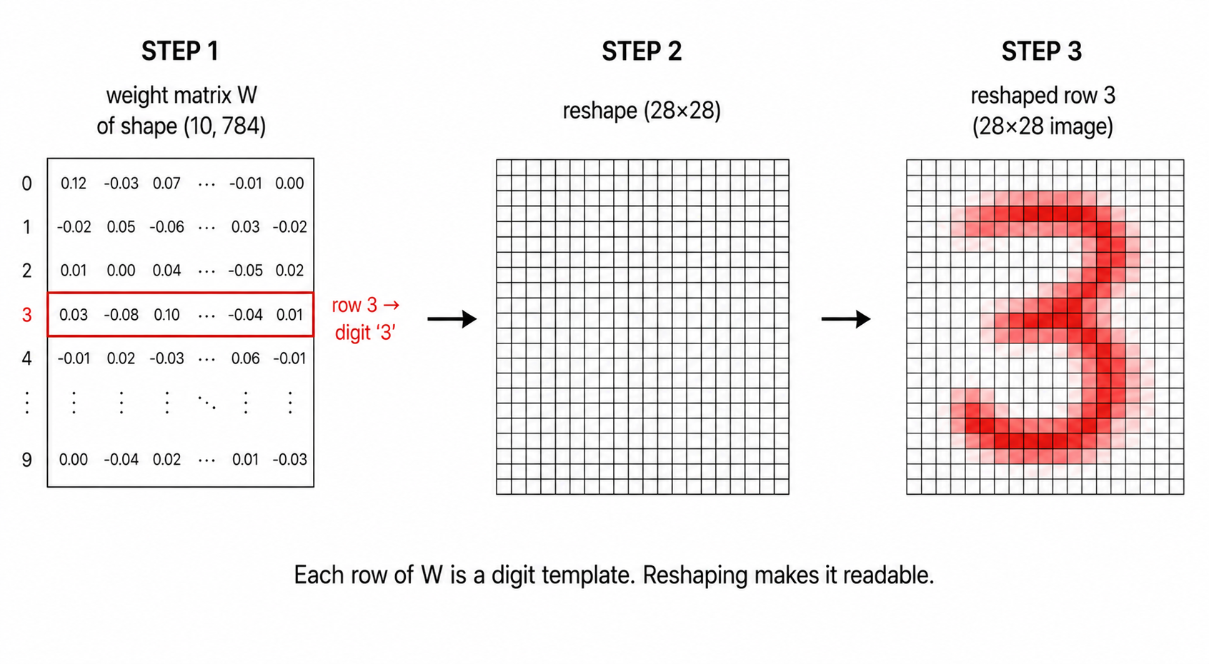
What you'll see: 10 images, each looking like a fuzzy digit. The row for class "0" looks like a hollow circular blob. The row for class "1" looks like a vertical stripe. And so on. These are the templates the model has learnt: it predicts the class whose template most resembles the input.
That's the entire algorithm. Logistic regression on MNIST is template matching. You can read this directly off the weights.
Experiment B: a tiny MLP, and the first hint of messiness
Now train a slightly bigger model: a 1-hidden-layer MLP (multilayer perceptron) with 32 hidden neurons. The first-layer weights are now a matrix of shape (32, 784) - 32 hidden neurons, each with a 784-dim "input filter".
Plot all 32 filters as 28×28 heatmaps. What you'll see: some look like edges and strokes (cleaner features than the templates), but many look messy - like blends of two or three digits, or patterns that don't have an obvious meaning. Some are barely active. Some are clearly multi-purpose.
That messiness is your first encounter with polysemanticity - the phenomenon where one neuron is involved in many features at once. It's the central puzzle of mech interp, and the entire next project (Toy Models of Superposition) is dedicated to understanding why it happens.
crack open as needed
Glossary - terms you'll meet here
If you're brand new to ML, some of these might be your first time seeing the word. Skim now, refer back as needed.
- Notebook: an interactive document where prose and runnable Python code cells are interleaved. Each step of this curriculum is rendered as a notebook - the page you're reading right now is one. Code cells have a Run button; everything else is just text.
- Vector: an ordered list of numbers. A 28×28 MNIST image becomes a vector of 784 numbers (one per pixel, read row by row). Both the input and the output of a neural network are vectors.
- Layer: a chunk of the network that takes a vector in and outputs a different (usually different-sized) vector. Stacking layers is how you build deeper models.
- Linear layer: the simplest possible layer - just one matrix multiplication plus a bias:
out = x @ W.T + b. No nonlinearity. Logistic regression is a single linear layer; an MLP is two or more linear layers with a nonlinearity (like ReLU) between them. - Bias: a small per-output offset added after the matrix multiply. Lets the layer shift its outputs up or down independently of the input.
- Neural network: a function from input vectors to output vectors, defined by a collection of learnable numbers (the weights). The function is built by stacking layers (linear maps, nonlinearities) on top of each other.
- Weights: the numbers inside the model. The thing training adjusts. Before training they're random; after training they're carefully tuned for the task. Everything we care about in interpretability lives in the weights.
- Logistic regression: the simplest kind of neural network. Literally one matrix multiply followed by a softmax. No hidden layer. The whole model is a single weight matrix
Wand a bias vectorb. - MLP (multilayer perceptron): logistic regression with one or more "hidden layers" stacked in between input and output, each followed by a nonlinearity. The first non-trivial neural network.
- Hidden layer: a layer of neurons between the input and the output. Called "hidden" because it's not directly observed during training - you only see input and output.
- Neuron: one scalar value (one number) inside a layer of the network. A layer is a vector of neurons. "100 hidden neurons" means the hidden layer is a 100-number vector. Each neuron's value is a weighted sum of the previous layer, optionally followed by a nonlinearity.
- Input pixel space: for MNIST, each image is 28×28 = 784 pixels. The input to the model is a length-784 vector.
- Class: one of the 10 possible labels (digit 0 through digit 9). The model predicts a probability distribution over classes.
- Softmax: a function that turns any vector of real numbers into a probability distribution (positive, sums to 1). Applied at the output of a classifier.
- Loss: a single number that measures how wrong the model is right now. Lower is better. We tune the weights to make it as small as possible.
- Cross-entropy loss: the specific loss we use for classification. Penalises low predicted probability for the correct class. You don't need to understand the formula yet; just know it's what you optimise.
- Gradient: for each weight in the model, "if I nudged this weight up a tiny bit, would the loss go up or down, and by how much?" The gradient is the collection of those answers, one per weight.
- Gradient descent: the algorithm that trains every neural network you'll ever meet. Start with random weights. Repeatedly: feed in data, compute the loss, compute the gradient, then nudge every weight a tiny step in the direction that decreases the loss. Thousands of steps later the weights have "descended" to a low-loss configuration. That's the whole show. Adam, AdamW, SGD - those are all just different recipes for how big a step to take.
- Backpropagation: the calculus trick that computes the gradient efficiently. In code it's literally one line:
loss.backward(). - Optimiser: the bit that actually applies the gradient-descent step. We'll use Adam, a sensible default. In code you'll see it spelled
optimizerbecause PyTorch uses American spelling. - Training loop: the cycle of (1) forward pass: model makes predictions, (2) compute loss, (3) compute gradients via backpropagation, (4) optimiser updates the weights. Repeat thousands of times.
- MNIST: short for Modified National Institute of Standards and Technology - a dataset of 70,000 28×28 greyscale images of handwritten digits, each labelled 0-9. Old, small, perfect for tutorials.
- Template matching: an algorithm that compares the input to a stored prototype and outputs how similar it is. As you'll see, that's essentially what logistic regression on MNIST does.
Just enough PyTorch to follow along
If you've never trained a model in PyTorch before, this is the place to learn the absolute basics. The notebook itself is heavily commented; this section gives you the conceptual scaffolding.
Tensors
A tensor is PyTorch's name for a multi-dimensional array (basically a NumPy array that can live on a GPU and track gradients).
x = torch.zeros(3, 4)         # 3×4 tensor of zeros
y = torch.randn(10, 784)      # 10×784 tensor of normal-distributed random numbers
z = x @ y.T                   # 3×10 - @ is matrix multiplication
Models as nn.Module
A model is a Python class that inherits from nn.Module. You declare the learnable parts in __init__ and the forward computation in forward:
class TinyModel(nn.Module):
    def __init__(self):
        super().__init__()
        self.W = nn.Parameter(torch.randn(10, 784) * 0.01)
        self.b = nn.Parameter(torch.zeros(10))

    def forward(self, x):
        return x @ self.W.T + self.b
nn.Parameter says "this is a learnable weight - track gradients for it, let the optimiser update it." That's the whole machinery.
We can also use nn.Linear(784, 10) which packages exactly this in one line.
The training loop
Every PyTorch training loop has the same skeleton:
for step in range(n_steps):
    logits = model(x)                       # 1. forward pass - predictions
    loss   = F.cross_entropy(logits, y)     # 2. compute loss
    optimizer.zero_grad()                   # 3. clear old gradients
    loss.backward()                         # 4. compute new gradients (backprop)
    optimizer.step()                        # 5. update weights
That's it. You don't need to understand backpropagation in detail - loss.backward() is one line of code that computes "if I nudged each weight, would the loss go up or down?" The optimiser uses that to take a step in the direction that decreases the loss.
Two helpers we'll use
torch.optim.Adam(model.parameters(), lr=...)- the standard "smart" optimiser. Treat as a recipe.F.cross_entropy(logits, targets)- the standard classification loss. Compares predicted scores against integer class labels.
Run it
The notebook is mnist_templates.ipynb.
01Setup
Imports + device + seed. Standard plumbing.
02Load MNIST
We use torchvision.datasets.MNIST to download the dataset (~10MB). We flatten each image to a 784-dim vector and stack them into one big tensor. No DataLoader - we just slice random mini-batches from this tensor each step, which keeps the code simple.
03Logistic regression - the simplest possible model
A LogReg module with one nn.Linear(784, 10). Train 5 epochs of Adam (mini-batches of 256), log loss and accuracy per epoch.
04Visualise the weights as digit templates
Reshape each row of W to 28×28 and plot. Each plot has the corresponding digit label. The wow moment.
Look closely. Red regions are positive weights (the model wants ink there for this class); blue regions are negative (the model wants ink absent there for this class).
You should see:
- "0": a red ring around the edge (where the loop of a 0 sits) with blue in the middle (since 0 has a hollow centre).
- "1": a vertical red stripe down the middle.
- "3", "8": stacked curves.
- "7": a red horizontal bar on top and a diagonal stroke.
Each template is a blurry average of all the training examples of that digit, sculpted by training to discriminate between classes.
This is the whole algorithm. Logistic regression on MNIST is template matching. The model takes your input image, dots it against 10 stored templates, and predicts the class whose template gave the highest dot product. You can read the whole algorithm directly off the weight matrix. This is interpretability in its simplest form.
05A 1-hidden-layer MLP
Same training loop but with one hidden layer of 32 ReLU (rectified linear unit) neurons in between. Roughly the same accuracy or slightly better.
06Visualise the MLP's first-layer weights
Reshape each of the 32 hidden neurons' input weights to 28×28 and plot in a grid. Compare to the clean templates from Section 4. The pivot to project 1.
Compare to Section 4. The logistic-regression templates were clean: one digit template per class, each visually recognisable.
The MLP's first-layer filters are messier. You'll likely see:
- Some filters that look like clean edges or strokes - parts of digits.
- Some that look like blurry blends of two or three digits at once.
- Some that look almost like random noise (or like a faint mix of many things).
- A few that look strikingly clean and others that don't.
Why are these messier? Because there are only 32 hidden neurons but a lot of useful features of digits a model could track - edges, curves, intersections, stroke directions, you name it. Each hidden neuron ends up doing several jobs at once, because there aren't enough neurons to give each useful feature its own dedicated neuron.
This is your first encounter with polysemanticity - one neuron firing for many unrelated features. It is the single biggest obstacle in modern mech interp, and it's why the next project (01-toy-models-superposition/) exists.