Learn mechanistic interpretability

This project is a small, friendly entry point into mechanistic interpretability - the field of "reverse-engineering" neural networks to figure out what algorithms they actually learnt. We partially replicate a famous Anthropic paper, Toy Models of Superposition (Elhage et al., 2022), in a single Jupyter notebook (toy_models_superposition.ipynb).

By the end you'll have:

Trained a tiny neural network from scratch in PyTorch.
Watched it learn to do something genuinely surprising: represent 5 features in only 2 dimensions by packing them into a pentagon.
Built intuition for "superposition", the central obstacle that modern interpretability research (sparse autoencoders, Anthropic's circuits work, Neel Nanda's tutorials) is trying to solve.

What is superposition? (the one big idea)

Here's the single concept this entire project is built around. It's worth understanding before touching the code.

First: what's a "feature"?

Before we can talk about how the model stores features, we need to be precise about what one is.

In mech interp, a feature is a hypothesised concept or property that a model has learnt to track internally. Think of features as the "variables" the network has invented for itself to make sense of its input. Some real examples from interpretability papers on language models:

"this token is inside a Python comment"
"this sentence is in French"
"this paragraph is about a dog"
"this character follows an open quote mark"
"this is a year between 1900 and 2000"
"the next token will be capitalised"

Two important properties:

A feature is not the same as a neuron. A feature is an abstract concept the network is tracking. A neuron is one specific scalar number inside the network. Mech interp is largely the question: how do the abstract features map onto the concrete neurons, weights, and attention heads?
Real-world features are sparse. At any given moment, almost all features are off. The sentence you're reading right now is not in French, not in a Python comment, not about a dog, not a year, etc. Out of the (thousands of) features a model might track, only a handful are active for any given input. This sparsity is what makes superposition possible.

In our toy project we don't bother making features represent real concepts. We just generate 5 abstract synthetic features - call them feature 0 through feature 4 - and ask the tiny model to compress and reconstruct them. These stand in for the rich features a real model would learn from real data. The question is purely: how does the model arrange them in its tiny 2-dimensional hidden space?

A quick note on "dimensions" and "hidden space"

Two pieces of geometry vocabulary you need before going further:

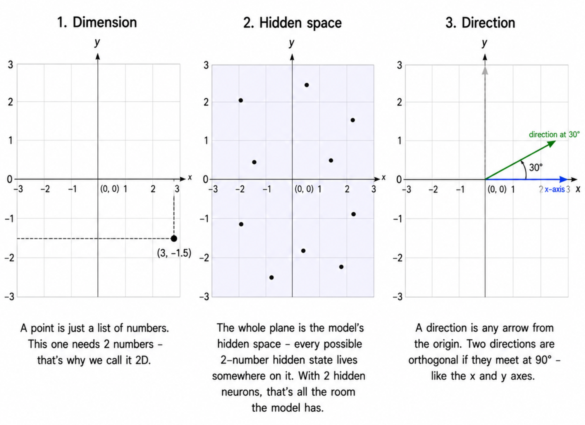
Dimension: one of the numbers in a vector. A point in 2D is two numbers like (3, -1.5). 3D is three numbers (x, y, z). 100D is 100 numbers - impossible to picture, but the maths works exactly the same.
Hidden space: the set of possible values inside the model's bottleneck layer. Our model has 2 hidden neurons, so any "hidden state" is just a pair of numbers - a single point you can literally draw on a page. That's exactly why we chose m=2 for this experiment: 2D is plottable.
Direction: any non-zero vector, pointing from the origin out into the space. Two vectors are orthogonal (perpendicular) if they form a 90° angle - like the x-axis and y-axis. Most pairs of random directions are not orthogonal; they overlap somewhat.

Real language models have hidden spaces of dimension 768, 4096, or even 12,288. You can't draw those, but each feature still gets a direction in that high-D space. Exactly the same idea as our 2D toy - just not visualisable.

A puzzle

Suppose I have a tiny network with 2 hidden neurons. How many distinct features can it represent?

Naively: 2 (one per neuron). At best: 2 orthogonal directions in the 2D hidden space - say, the x-axis and the y-axis. Anything more and the directions would have to overlap, causing interference.

Surprise: real networks routinely represent way more features than they have neurons. A model with 100 hidden neurons might represent thousands of features. How?

The trick

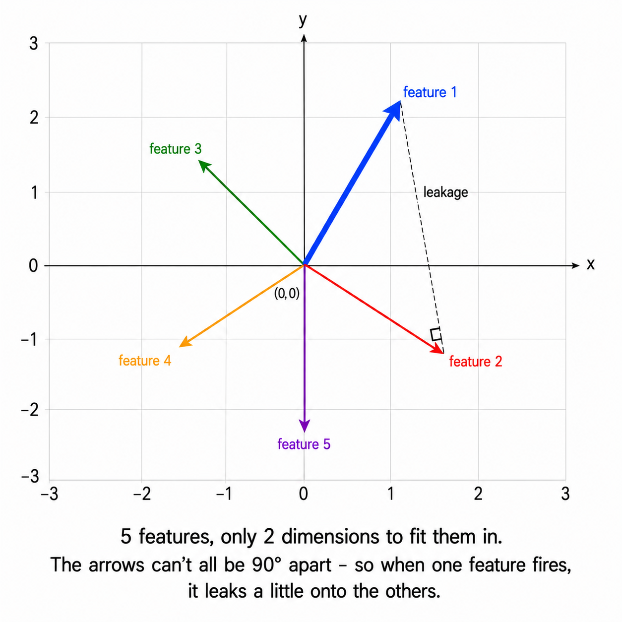
The model represents each feature as a direction in hidden space. The directions can't all be orthogonal - there aren't enough orthogonal directions to go around. So they overlap a little. When feature A is active, it slightly "leaks" into the direction for feature B.

(You'll actually see what these directions look like in the notebook - the headline experiment plots each feature's direction as an arrow in the 2D hidden plane.)

This sounds catastrophic, but two things save the model:

Features are sparse. In real data, most features are zero most of the time. The word you're reading right now is not in a Python comment, not in Japanese, not about the Golden Gate Bridge, not a date, etc. - almost all features are off. So two features rarely fire together, and interference is rare.
ReLU clips the leakage. When feature A leaks a small positive value into feature B's output, the ReLU (or really any nonlinearity) can clip it down to zero. The model learns to use this.

The result: a network can pack n >> m features into m neurons, as long as features are sparse enough. This is superposition.

Why this matters for interpretability

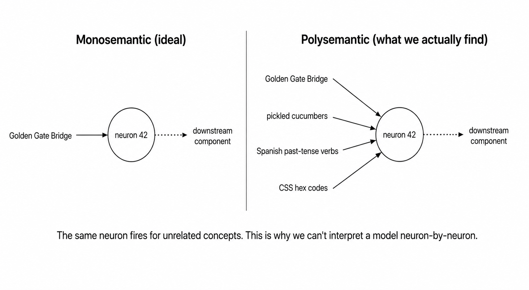
If features are stored in superposition, then individual neurons are polysemantic - one neuron lights up for many unrelated features at once. You can't understand the model by looking at neurons one by one. You have to find the directions in activation space that correspond to single, clean features.

Monosemantic vs polysemantic neuron: on the left, a single 'Golden Gate Bridge' input feeds into neuron 42; on the right, four unrelated inputs (Golden Gate Bridge, pickled cucumbers, Spanish past-tense verbs, CSS hex codes) all feed into the same neuron 42.

This is exactly the problem sparse autoencoders (SAEs) are trying to solve. Superposition is the headline obstacle in modern interp.

In this project we don't go all the way to SAEs - we just see superposition emerge in the simplest possible setting.

The experiment in plain English

Here's the whole experiment, before any code.

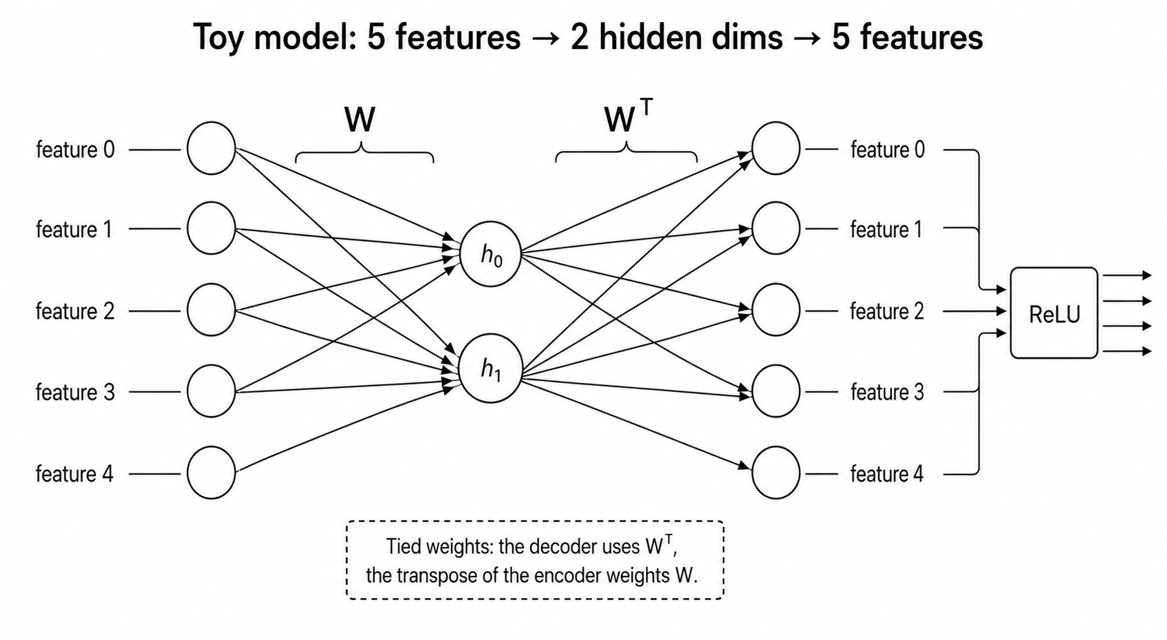
The model. Take n real-valued features (say n = 5) and an even tinier hidden layer of size m (say m = 2). The model has to compress the input down to m dimensions and then reconstruct it. It's an autoencoder with a bottleneck:

input (5)  →  hidden (2)  →  output (5)

The weights going down and coming back up are tied - the same matrix W is used (transposed) for both. So there's really just one weight matrix W of shape (2, 5) to learn. Plus a tiny output bias.

The output is passed through a ReLU (i.e. max(0, x)).

Toy model architecture: 5 input feature nodes on the left, fully connected via W to 2 hidden nodes h0 and h1 in the middle (the bottleneck), then fully connected via W transpose to 5 output feature nodes on the right, with a ReLU applied at the end. Note: the decoder uses the transpose of the encoder weights - tied weights.

The data. Synthetic. For each input vector:

Each of the 5 features is "active" with some probability 1 − S (where S is the sparsity).
If active, its value is a random number in [0, 1].
If inactive, it's exactly 0.

So S = 0 means features are always on (dense). S = 0.99 means only ~1 in 100 features is on (very sparse, like real data).

The loss. Importance-weighted mean squared error between input and reconstruction. Feature i gets importance 0.7^i, so feature 0 is the most important and the model will preferentially represent it.

The experiment. Train fresh copies of the model at increasing sparsity levels: S ∈ {0, 0.7, 0.9, 0.97, 0.99}. After training, plot the columns of W as arrows in 2D space. Each arrow is the 2D direction the model uses to represent that feature.

The reveal. At S = 0 (no sparsity), only the 2 most important features get represented - two perpendicular arrows, the others collapse to zero. At S = 0.99, all 5 features show up as a regular pentagon - 5 equally-spaced directions. The model figured out how to pack 5 features into 2 dimensions, because it knows they almost never co-occur.

crack open as needed

Glossary - terms added in this step

Skim these now; refer back as needed. Everything you'll meet in the rest of the README is defined here in one place.

Geometry

Dimension - one of the numbers in a vector. A 2D space = each point is 2 numbers; 100D = 100 numbers.
Vector - an ordered list of numbers. In this project, both inputs and hidden states are vectors.
Direction - a non-zero vector pointing out from the origin. We care about the direction of W's columns, not just their length.
Orthogonal - at 90° to each other. The x-axis and y-axis are orthogonal. Two orthogonal directions don't interfere.
Activation space - the space of all possible values at some layer of the network. Our model has a 2D activation space at its hidden layer.
Hidden space / hidden layer - same thing as the bottleneck: the middle layer where the model has compressed its input. Ours is 2-dimensional.

Mech interp concepts

Neuron - a single scalar (one number) sitting in a layer of the network. A layer is a vector of neurons; "100 hidden neurons" just means the hidden layer is a 100-number vector. Each neuron's value is produced by taking a weighted sum of the previous layer plus an optional nonlinearity. Our model has 5 input neurons, 2 hidden neurons (h0, h1), and 5 output neurons.
Feature - a hypothesised concept or property the model is tracking internally. E.g. "this text is in French" or "this token is a number." In our toy model we use 5 abstract synthetic features that stand in for real ones. Features ≠ neurons - features are abstract concepts, neurons are concrete scalar slots. One neuron can be involved in many features at once (that's the whole point of superposition).
Superposition - representing more features than dimensions, by packing them into non-orthogonal directions and exploiting the fact that features are usually sparse. The phenomenon this whole project demonstrates.
Polysemantic neuron - a neuron that fires for many unrelated features at once. The default state of neurons in models that use superposition. Makes interpretation hard.
Monosemantic feature - a single direction in activation space that corresponds to one clean concept. The interpretability goal.
Sparse autoencoder (SAE) - a wider autoencoder with a sparsity penalty, trained on a real model's activations, in the hope of recovering monosemantic features. The natural follow-up to this project.

Model anatomy

Autoencoder - a model that tries to reconstruct its own input after passing it through a smaller intermediate representation.
Bottleneck - the narrow middle layer in an autoencoder. The thing that forces the model to compress.
Tied weights - using the same matrix (transposed) for both encode and decode. Our model is tied; this halves the parameter count and is what the paper uses.
ReLU - max(0, x). The nonlinearity at the end of our forward pass. Defined in step 0; in this project its job is to clip the cross-talk that allows superposition to work (see The trick above).
Importance weight - how much a feature contributes to the loss. We use a geometric decay (0.7^i) so feature 0 matters most.

Data / training concepts

Sparsity (S) - probability a feature is zero in any given input. S=0 → dense; S=0.99 → very sparse.
Feature density - 1 − S, the probability a feature is on. The x-axis of the phase-transition plot.
MSE loss - mean squared error, mean((prediction − target)²). The standard reconstruction loss.
Importance-weighted MSE - MSE where each feature's error is multiplied by its importance.

Adjacent concepts you'll bump into

PCA - principal component analysis. Finds top-k orthogonal directions of variance in data. A model with no nonlinearity and dense features will basically learn PCA - exactly what you'll see at S=0.
Circuit - a small, identifiable subgraph of a neural network that implements an interpretable algorithm. Not in this project, but the goal of mech interp more broadly.

run it

The notebook is toy_models_superposition.ipynb. Each numbered section below maps to a section in the notebook.

01Setup

Import PyTorch, NumPy, matplotlib. Pick cuda if available, else CPU. Seed the RNGs for reproducibility. Nothing interesting here - just plumbing.

code · python

02The model

Defines ToyModel, the tiny autoencoder. The forward pass is essentially three lines:

hidden = x @ self.W.T            # (batch, n_features) @ (n_features, n_hidden) → (batch, n_hidden)
out    = hidden @ self.W + self.b # back up to (batch, n_features)
return F.relu(out)

Note: W has shape (n_hidden, n_features) - that is, each column of W is the direction in hidden space for one feature. That's what we'll plot later.

The ReLU at the end is doing real work: it's what makes the model able to do superposition. Without it, this would just be PCA.

code · python

03Synthetic data - sparse features

A simple function generate_batch that produces sparse non-negative feature vectors. Each feature is independently on with probability (1 - sparsity). Worth running and inspecting at a couple of sparsity values to build intuition for what the inputs look like.

code · python

04Feature importance and loss

Two helpers:

make_importance(n_features) - returns [1, 0.7, 0.49, 0.343, ...], a geometrically decaying importance per feature.
loss_fn(out, target, importance) - importance-weighted MSE. Important features get higher weight in the loss.

This is the lever that makes the dense (S=0) case interesting: with no sparsity, the model has to choose which 2 features to represent, and importance tells it which two.

code · python

05Training loop

A train() function that creates a fresh model, trains it for 10,000 steps using AdamW with a cosine learning-rate schedule, and returns the trained model plus the loss curve. The smoke test cell trains one model at sparsity=0.9 and plots the loss curve on a log scale. You should see the loss drop by about 2 orders of magnitude - that's training working.

code · python

Smoke test: train one model and check the loss curve

Let's verify training works at all. We expect to see the loss drop by ~2 orders of magnitude over training.

code · python

06The headline experiment: sweep over sparsity

This is the meat of the project. We train 5 fresh models, one at each sparsity level in [0.0, 0.7, 0.9, 0.97, 0.99]. For each one, we plot the 5 columns of W as arrows in the 2D hidden plane.

plot_W() is a small matplotlib helper - for each feature, draw an arrow from the origin to (W[0, i], W[1, i]). Colour the arrows by feature index so you can tell which is which.

The output is a row of 5 small panels, one per sparsity level. This is the figure to compare with the original paper.

code · python

07Discussion: what just happened?

A markdown cell that interprets the plot in words. Read this after you've seen your own output, then compare it to the description.

08Stretch goal: feature dimensionality

A neat follow-on experiment. We define a per-feature quantity D_i (defined in the notebook) that measures "what fraction of a hidden dimension does feature i get?" It's bounded between 0 and 1, with specific rational values for known geometries: 1 for orthogonal, 1/2 for antipodal pairs, 2/3 for a triangle, 2/5 for a pentagon vertex, 0 for not represented at all.

We then train ~25 models across a fine grid of sparsity values and plot D_i against sparsity. The result has discrete plateaus at those rational values - sharp phase transitions between geometries as sparsity changes. It's one of the prettier figures in the paper.

code · python

09Where to go from here

Suggestions for follow-ups - staying in the toy model, or stepping up to real transformers via Neel Nanda's TransformerLens.

How to run it

Go to colab.research.google.com.
File → Upload notebook → upload toy_models_superposition.ipynb.
Runtime → Change runtime type → GPU (T4 is fine and free).
Runtime → Run all. Total runtime:for the main experiment, anotherif you run the stretch section.

No installation needed - Colab comes with PyTorch and matplotlib pre-installed.

If you'd rather run locally, you need Python 3.10+, torch, numpy, and matplotlib. CPU is fine; the whole thing runs in a few minutes.

Where to go next

Next in the curriculum: 02-grokking-modular-addition/ - meet your first transformer, and watch it learn an actual algorithm. The features you just learnt about (now in 128 dimensions, packed in superposition) will be lurking inside its embedding matrix.

Sequel project at the end of the series: 05-sparse-autoencoders/ - the field's current best answer to the superposition problem we just diagnosed. We train a sparse autoencoder to automatically recover the feature directions out of a superposed model.