This is project 2 in our mech interp series. We replicate the core finding of Progress Measures for Grokking via Mechanistic Interpretability (Nanda, Chan, Lieberum, Smith, Steinhardt - 2023), one of the most striking results in mech interp.
By the end you'll have:
- Trained a tiny 1-layer transformer on a simple maths problem and watched it do something genuinely strange: sit at ~chance performance for thousands of training steps, then suddenly "wake up" and generalise perfectly.
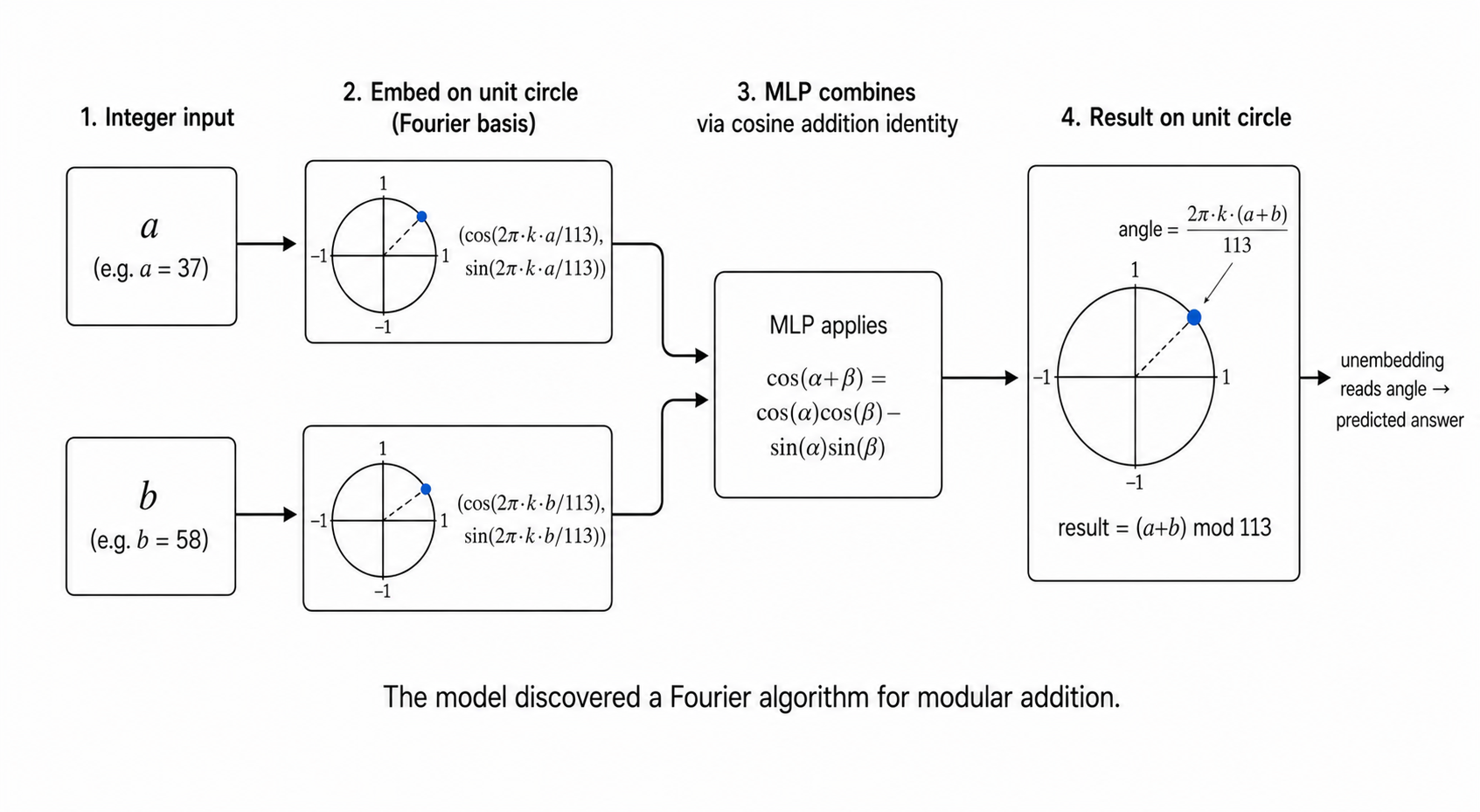
- A mechanistic explanation for that delayed generalisation - you'll look inside the trained model and discover it learnt a trigonometric algorithm based on the Fourier basis. ("Fourier" is the idea that any repeating pattern can be written as a sum of sines and cosines at different frequencies. In this project, the model uses sines and cosines to represent numbers as rotations around a circle - because the task wraps modulo 113, "rotations" is the natural way to think about it.)
- Your first transformer, built from scratch in PyTorch.
This is the spiritual successor to project 1 (Toy Models of Superposition). Same recipe - train a small model from scratch, then reverse-engineer it - but now we get to use a transformer.
What is grokking?
In normal supervised learning, a model's training loss and test loss both improve together. The model gets better at the data it has seen and better at unseen data, in lockstep, roughly.
Grokking is what happens when those two curves come apart in a really weird way:
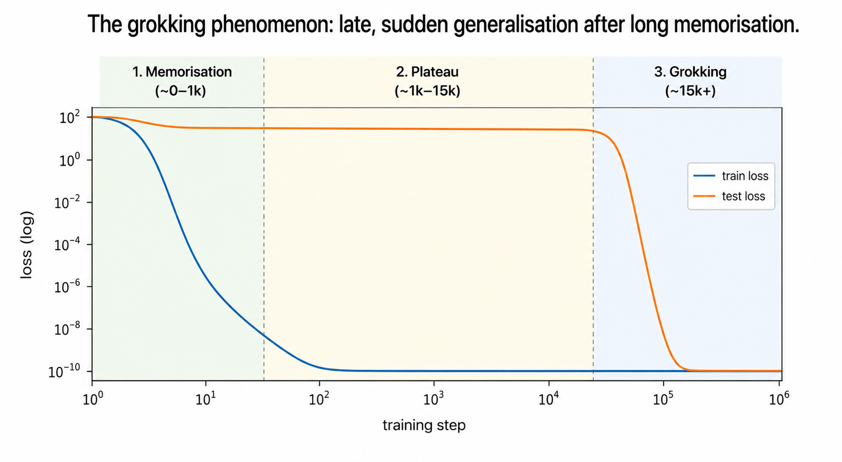
- Memorisation phase (steps 0 → ~1k): training loss drops to near zero - the model has memorised the answers to every training example. Test loss stays at chance level - the model has learnt nothing generalisable.
- Plateau (steps ~1k → ~10k+): training loss stays low, test loss stays bad. Looks like the model has just memorised and that's it. For a long, long time.
- Grokking (suddenly, much later): test loss falls off a cliff and reaches near-zero. The model has, somehow, figured out the underlying rule and now generalises perfectly - long after it could have just stopped at memorisation.
This was first reported by Power et al. 2022 ("Grokking: Generalisation Beyond Overfitting on Small Algorithmic Datasets") at OpenAI. They observed it but had no mechanistic explanation.
Nanda et al.'s 2023 paper took the same setup, fully reverse-engineered the trained model, and showed exactly what was happening: during the "boring" plateau, the model was slowly building up a generalising circuit alongside the memorised solution. When the circuit got good enough, it took over.
That circuit is what makes this whole thing beautiful - it's a clean, human-understandable algorithm based on Fourier series. We'll find it.
The task: modular addition
The model learns to add two numbers modulo a prime p.
Pick p = 113. The model sees three input tokens - a, b, = - where a, b ∈ {0, 1, ..., 112}, and has to predict the answer (a + b) mod 113 at the = position.
Examples:
- input
(0, 0, =)→ answer0 - input
(5, 10, =)→ answer15 - input
(100, 50, =)→ answer37(because150 mod 113 = 37) - input
(112, 1, =)→ answer0(the "wrap-around")
There are 113 × 113 = 12,769 total possible (a, b) pairs. We train on a random 30% of them and test on the remaining 70%. With this setup, the model has plenty of room to overfit (memorise the 30%) but only generalises if it learns the actual rule.
The choice of p being prime matters - it makes the maths have nice Fourier structure, which is what the model ends up exploiting.
The experiment in plain English
The whole experiment, before any code:
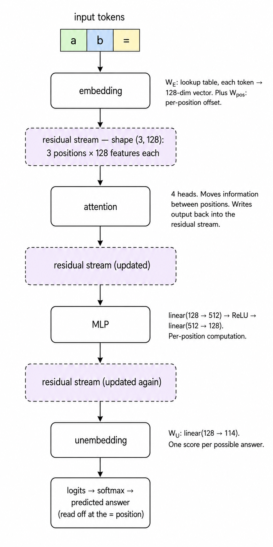
The model. A 1-layer transformer with 4 attention heads, hidden size d_model=128, MLP hidden size d_mlp=512. No layer norm, no dropout (we want the cleanest possible mech-interp target). Total parameters: ~200k. Tiny by modern standards but plenty for this task.
The data. All 113 × 113 = 12,769 pairs (a, b), each labelled with (a+b) mod 113. We split randomly into 30% train, 70% test.
Training. AdamW with learning rate 1e-3 and weight decay 1.0 (this is large - weight decay is doing serious work here). Full-batch (we use all 3,830 training examples per step). Cross-entropy loss on the prediction at the = position.
What we plot. Train loss and test loss vs step, both on a log scale, for ~25,000 steps. You should see:
- Train loss crashes to near zero within the first ~500 steps. (Memorisation)
- Test loss stays bad - close to
log(113) ≈ 4.7, which is the loss of random guessing among 113 classes - for a long time. - Then, somewhere around step 10,000–20,000, test loss falls off a cliff and reaches near zero. (Grokking - the wow moment.)
The reverse-engineering (stretch). We take the trained model's embedding matrix W_E (shape (d_vocab, d_model) - one vector per number 0..112 plus =). We do a discrete Fourier transform along the vocab dimension. We discover that almost all of the embedding energy lives in just a handful of Fourier frequencies - the model is representing each number as cos(2πkx/p) and sin(2πkx/p) for a small set of k. This is the Fourier algorithm the model has discovered, sitting right there in the embedding weights.
Why does this work mathematically? The trig identity:
cos(2π·k·(a+b)/p) = cos(2π·k·a/p) · cos(2π·k·b/p) − sin(2π·k·a/p) · sin(2π·k·b/p)
If the model represents a and b as Fourier features, an MLP can implement that identity using multiplications and combinations. Then the unembedding reads out the answer at the right frequency. The whole thing is a clean, human-understandable algorithm - built by SGD, not by us.
crack open as needed
Glossary - terms added in this step
Just the new ones. For earlier terms (feature, direction, dimension, superposition) see the step 1 glossary.
Grokking-specific
- Grokking: late, delayed generalisation. The phenomenon this project is about.
- Memorisation: the model perfectly fits training data without learning a rule. Looks like learning but doesn't transfer to new examples.
- Generalisation: the model performs well on examples it has never seen - evidence that it learnt the underlying rule, not the table of answers.
- Train / test split: a random partition of the data. The model only ever sees the train half during training; the test half is used to measure whether it actually learnt a generalising rule.
- Weight decay: a regularisation technique that pulls weights toward zero. Crucial for grokking - without weight decay, grokking does not happen. We'll explain why below.
- AdamW: the variant of the Adam optimiser that implements weight decay correctly. Just use it; you don't need to understand the details. (In code you'll see it spelt
optimizerbecause PyTorch uses American spelling.)
Transformer anatomy
- Token: a single discrete input symbol. In our setup, the vocabulary is 114 tokens (
0,1, …,112,=), and each input sequence has 3 tokens (a,b,=). - Vocabulary (
d_vocab): how many distinct tokens exist. For us,114. - Embedding (
W_E): a learnable lookup table that maps each token to a vector of sized_model. The very first thing the model does to your input. - Positional embedding (
W_pos): a small learnable vector added per position in the sequence - lets the model tell apart "this is the first input" vs "this is the second input." - Residual stream: the running vector at each position as it flows through the layers. The transformer's "main bus" - every component reads from it and writes back into it.
- Attention head: a component that lets the model mix information across positions. We have 4 heads in 1 layer.
- MLP (multilayer perceptron): a simple stack of linear layers with a nonlinearity in between (
linear → ReLU → linear). Sits after attention and does per-position computation. - Unembedding (
W_U): a final linear layer that maps thed_model-sized vector back tod_vocablogits - one score per possible output token. The model picks the one with the highest score. - Logits: the raw, unnormalised scores the model outputs. Softmax of the logits gives a probability distribution over tokens.
- Cross-entropy loss: the standard classification loss - penalises low predicted probability for the correct answer.
Mech interp / Fourier
- Fourier basis: a way of writing any function on
{0, 1, ..., p-1}as a sum of sines and cosines at different frequencies. The mathematical structure the model ends up using. - Frequency: an integer
kindexing one of the trig functionscos(2πkx/p),sin(2πkx/p). Withp=113, valid frequencies are0through56. - Progress measure: a quantity you can compute from the model's weights that smoothly increases even during the "flat" plateau. Reveals that the model is slowly building its circuit underneath, even when the test loss isn't dropping.
Just enough transformer to follow along
You did project 1, so you already know nn.Module, nn.Parameter, the training-loop skeleton, ReLU, loss, optimiser. The new concept here is the transformer.
A transformer is just a particular arrangement of standard neural-net pieces (linear layers, ReLU, softmax). Here's the entire architecture in one diagram, conceptually:
Three concepts you need to internalise:
5.1 The residual stream
The transformer keeps a running (n_positions, d_model) tensor that flows through the layers. For us this is (3, 128) - three positions (one for a, one for b, one for =), each holding a 128-dim vector.
Every component (embedding, attention, MLP) reads from this tensor and adds its output back into it. Nothing is destructively overwritten. This is the "residual" part - outputs are added, not replaced.
Think of the residual stream as the model's working memory: a shared whiteboard that every component reads from and writes to.
5.2 Attention
An attention head's job is to move information between positions. In our setup, it's the only mechanism that lets the model combine information about a (at position 0) and b (at position 1) into a single computation at the = position (position 2). The MLP, by contrast, only operates within one position at a time.
Each head has four small matrices: W_Q (query), W_K (key), W_V (value), W_O (output). The mechanics:
- For each position, the head computes a query (
q = W_Q @ residual) and a key (k = W_K @ residual). - For each pair of positions, it computes an attention score:
score[i, j] = q_i · k_j. - It softmaxes the scores along the source dimension to get attention weights (each position's "attention" sums to 1).
- It computes values (
v = W_V @ residual) and outputs a weighted sum of values, weighted by the attention weights. - It projects back via
W_Oand adds the result into the residual stream.
You don't have to memorise this. The mantra is: attention moves information between positions; everything else runs within a position.
5.3 Weight decay (and why it matters for grokking)
Weight decay is a regularisation technique: at every optimiser step, in addition to the gradient update, it pulls all weights slightly toward zero. Mathematically: w ← w - lr · gradient - lr · weight_decay · w.
Why does this matter for grokking? Roughly: there are two ways to solve the task.
- Memorisation: store a giant lookup table of (a, b) → answer in the weights. This works perfectly on the train set but uses a lot of weight "mass."
- Generalisation: learn a small, clean Fourier algorithm. Uses very little weight mass.
Without weight decay, the model is happy to sit at memorisation forever - both solutions get loss 0 on train, and there's no pressure to find the cleaner one. With weight decay, big-weight memorisation is penalised. The model has to slowly carve out the smaller, cleaner generalising solution. That carving is what we see as the long plateau, and grokking is the moment the cleaner solution becomes good enough to take over.
This is why the paper is called Progress Measures - even during the plateau, weight decay is slowly squeezing weight mass from the memorised solution into the generalising one. The progress is real but invisible in the loss curves until the crossover.
Run it
The notebook is grokking.ipynb. Each section below maps to a section in the notebook.
01Setup
Imports, device, seeds. Same as before.
02Hyperparameters
A single cell of constants - p = 113, d_model = 128, n_heads = 4, d_head = 32, d_mlp = 512, train_frac = 0.3, weight_decay = 1.0, n_steps = 25_000, etc. Keeping them in one place makes experiments easier.
03The data
Generate all p² pairs (a, b) with their labels (a+b) mod p. Format each example as a length-3 sequence [a, b, p] where token p is used as the = marker (we just stuff = into the same vocab as a 114th token at index p). Random shuffle, take the first 30% as train.
04The transformer
A hand-rolled tiny transformer in ~50 lines of PyTorch. We define:
- An
Embedding(token + position). - An
Attentionlayer with 4 heads. We use rawQ, K, V, Olinear layers; you'll be able to inspect them later. - An
MLPlayer (linear → ReLU → linear). - A
Transformerclass that stacks them, applies the unembedding, returns logits at the=position.
Hand-rolled is the mech-interp tradition - using nn.Transformer would hide the internals we want to inspect.
4b. MLP
The MLP runs independently at each position. It's just linear → ReLU → linear.
4c. Putting it together
Embedding → attention (with residual) → MLP (with residual) → unembedding.
Note we deliberately omit LayerNorm - the paper omits it too. It makes the mech interp analysis much cleaner because the residual stream isn't being repeatedly rescaled.
05Training
Standard loop, AdamW, cross-entropy on the =-position logits. Every 100 steps we record both train loss and test loss, so we can plot them at the end.
Heads up: this is the slow cell. The default is 10,000 steps of full-batch training, so on a T4 GPU it takes around 4 minutes to finish. It's slow because every step does a forward + backward over the entire training set (~3,800 examples) rather than a mini-batch - that's deliberate, because grokking is sensitive to optimiser noise and full-batch makes the phase transition clean and reproducible. Don't navigate away from this page while it's running - the kernel is stateful, so closing the tab kills the in-flight training and leaves later cells without the trained model to inspect.
06The grokking curve - the wow moment
The headline plot. Train loss vs test loss vs step, log scale. This is the wow moment. You'll see the train loss crash to zero almost immediately, then a long flat plateau on test loss, then a sudden cliff. We mark the rough memorisation phase, plateau, and grokking phase on the plot.
07Stretch: Fourier analysis of the embedding
We take the trained W_E matrix and do an FFT along the vocabulary axis. We then plot the magnitude of each Fourier component across hidden dimensions. The plot should show that energy is concentrated in just a handful of frequencies - the model has rediscovered the Fourier basis.
What you should see
Most of the bars near zero, with a small number of "spikes" at specific frequencies. Those spikes are the model's chosen frequencies - the model represents each number x as [..., cos(2π·k·x/p), sin(2π·k·x/p), ...] for k in that small set.
The full mech interp story (which we don't replicate in this notebook) is that:
- The embedding rotates each number
xinto a Fourier basis. - The MLP uses its quadratic-ish structure (linear → ReLU → linear) to implement the product-to-sum trig identity
cos(2πk(a+b)/p) = cos(2πka/p)·cos(2πkb/p) − sin(2πka/p)·sin(2πkb/p). - The attention head shuffles information from positions 0 and 1 (where
aandblive) onto position 2 (the=). - The unembedding reads out the result, peaked at the correct answer.
What you just discovered (a sparse Fourier spectrum in W_E) is the first piece of evidence for step 1. The full circuit reverse-engineering is a great next project - Neel's grokking demo Colab walks through it.