Learn mechanistic interpretability

Step 5 of 6 in the mech interp curriculum. Assumes you've done steps 0-4. (You especially need step 1, which set up the problem this step solves.)

We replicate the core idea of Sparse Autoencoders Find Highly Interpretable Features in Language Models (Cunningham, Ewart, Riggs, Huben, Sharkey; 2023) and Towards Monosemanticity (Bricken et al., Anthropic, 2023).

The ONE new idea this step teaches: you can automatically discover the features a model uses, by training a separate "interpreter" model (a sparse autoencoder) on the original model's hidden activations. No hand-crafted prompts, no head-by-head patching - just train an SAE and read the dictionary it learns.

This step closes the loop on the whole curriculum. Step 1 introduced superposition as the central obstacle of mech interp. Step 5 introduces SAEs, the field's current best partial solution.

By the end you'll have:

Trained a toy model that uses superposition (a slightly bigger version of step 1's setup).
Trained a sparse autoencoder on the model's hidden activations.
Verified that the SAE's learnt features recover the original model's ground-truth features - by cosine similarity, not by hand.

Why this step exists

Step 1 named the problem: real models pack features in superposition, so individual neurons stop being interpretable. Steps 2–4 worked around that - finding circuits by hand, verifying them by hand. This step automates the feature-finding part.

The pitch for an SAE in one sentence: train a wider autoencoder on the model's hidden activations, with a sparsity penalty, and the directions it learns will be the model's actual features.

What is a sparse autoencoder?

A sparse autoencoder is a small neural network with three pieces:

input x (d_input dims)
       │
       ▼
   ┌──────────┐
   │ encoder  │  W_enc, b_enc  → ReLU
   └──────────┘
       │
       ▼
hidden h (d_sae dims)   ← d_sae > d_input  (the dictionary; many more "features" than the input has dimensions)
       │
       ▼
   ┌──────────┐
   │ decoder  │  W_dec
   └──────────┘
       │
       ▼
output x̂ (d_input dims)

Forward pass:

h = ReLU(W_enc @ x + b_enc)
x̂ = W_dec @ h + b_dec

Loss:

L = ||x - x̂||²    (reconstruction - must faithfully decompose the input)
  + λ ||h||₁      (sparsity - penalises the number of features used)

The ReLU on h is essential - it means each feature can be off (h_i = 0) or active to varying degrees (h_i > 0), but never negative. Combined with the L1 penalty, the SAE is pushed toward solutions where most features are off and only a few fire on any given input.

After training, each column of W_dec is one feature direction in the input activation space. The SAE has learnt a dictionary of d_sae directions, and represents each input activation as a sparse, non-negative combination of those directions.

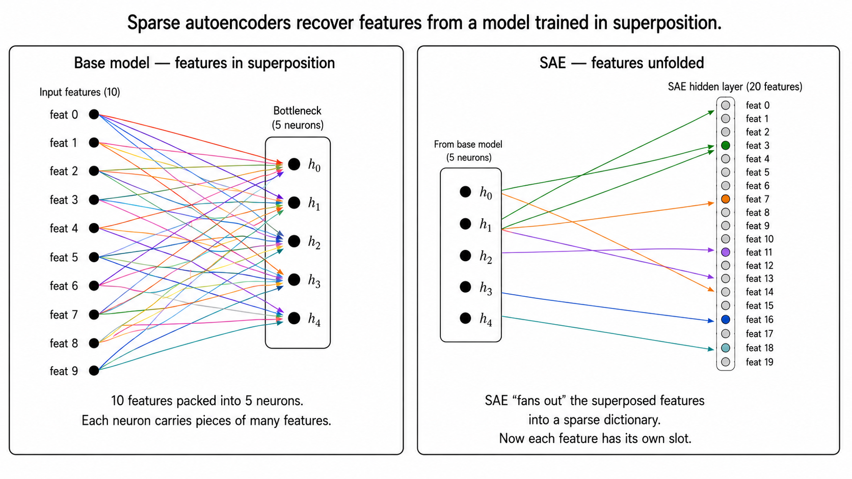
This is what fixes the superposition problem. The original model packs many features into fewer dimensions (project 1). The SAE projects back out into a higher-dimensional space where each feature can have its own dedicated dimension.

The experiment in plain English

We want to verify, in a setting where we have ground truth, that an SAE actually finds the real features.

The setup: train a project-1-style toy superposition model. Specifically:

n_features = 10 (the ground-truth features)
n_hidden = 5 (the bottleneck dimension)
sparsity = 0.9 (90% of features off on average)

This model packs 10 features into 5 hidden dimensions. We know the ground-truth feature directions: they're the 10 columns of the model's W matrix.

The SAE: train a sparse autoencoder on the model's hidden activations.

Input: 5-dim (the model's hidden state)
SAE width: 20 features (overcomplete by 4×)
Sparsity: L1 coefficient λ = 0.001

The test: after the SAE has trained, compute the cosine similarity between each SAE feature direction and each ground-truth feature direction. Build a 20×10 matrix and plot it. If the SAE has recovered the features:

Each ground-truth feature should be matched by at least one SAE feature with cosine similarity ≈ 1.
The SAE features not matched to any ground-truth feature are "dead" or redundant - that's normal.

This is the wow moment: the SAE didn't know about the 10 ground-truth features. It only ever saw 5-dim hidden activations from a trained model. With nothing but the L1 penalty as guidance, it recovers the original feature decomposition.

crack open as needed

Glossary - terms added in this step

Sparse autoencoder (SAE): an autoencoder whose hidden layer is wider than its input, trained with a penalty that forces only a few hidden units to fire on any given input. The "wider hidden than input" part is essential: if the hidden layer is the same size as the input, the obvious solution is the identity function and no features get found.
Dictionary learning: the general field of "find a sparse representation of data as combinations of basis elements." SAEs are a specific neural-network version. The "dictionary" is the set of basis elements (= the SAE's decoder columns).
Encoder / decoder: the two halves of an autoencoder. Encoder maps input → hidden (the dictionary coefficients). Decoder maps hidden → output (a reconstruction).
L1 penalty / L1 loss: a loss term proportional to the sum of absolute values of the hidden activations. Penalises any nonzero activation, so the optimiser prefers solutions that use as few hidden units as possible.
Reconstruction loss: the standard MSE between the SAE's output and its input. The SAE has to faithfully reproduce the original activation.
Feature direction (in an SAE): a column of the decoder weight matrix. The SAE represents each input as a sparse positive combination of these directions.
Monosemantic feature: a feature direction that, by inspection, corresponds to one clean concept. The interpretability goal. Project 1 defined this term; step 5 makes it operational.
Feature splitting: when a wider SAE breaks one "feature" from a smaller SAE into several finer ones. A phenomenon you'll see in larger setups; we don't focus on it.
Sparsity coefficient (λ): the weight on the L1 penalty in the SAE's loss. Higher λ → fewer features active per input but worse reconstruction. Picking this is the main SAE-training hyperparameter headache.

run it

The notebook is sparse_autoencoders.ipynb.

01Setup

Imports, device, seed.

code · python

02Train a superposition model (the "base model")

A slightly bigger version of step 1's ToyModel. We train it briefly at high sparsity so it packs 10 features into 5 hidden dimensions via superposition.

code · python

N_FEATURES = 10
N_HIDDEN   = 5
SPARSITY   = 0.9

class ToyModel(nn.Module):
    def __init__(self, n_features, n_hidden):
        super().__init__()
        self.W = nn.Parameter(torch.empty(n_hidden, n_features))
        nn.init.xavier_normal_(self.W)
        self.b = nn.Parameter(torch.zeros(n_features))

def encode(self, x):                      # x: (B, n_features) → (B, n_hidden)
        return x @ self.W.T

def forward(self, x):
        return F.relu(self.encode(x) @ self.W + self.b)

def make_sparse_batch(B, n_features, sparsity, device):
    vals = torch.rand(B, n_features, device=device)
    mask = torch.rand(B, n_features, device=device) > sparsity
    return vals * mask

def importance(n_features, device):
    return 0.7 ** torch.arange(n_features, device=device, dtype=torch.float32)

base = ToyModel(N_FEATURES, N_HIDDEN).to(device)
imp  = importance(N_FEATURES, device)
opt  = torch.optim.AdamW(base.parameters(), lr=1e-3)
sched = torch.optim.lr_scheduler.CosineAnnealingLR(opt, T_max=10_000)

for step in range(10_000):
    x = make_sparse_batch(1024, N_FEATURES, SPARSITY, device)
    loss = (((base(x) - x) ** 2) * imp).mean()
    opt.zero_grad(); loss.backward(); opt.step(); sched.step()
    if step % 2000 == 0:
        print(f'  base step {step:5d}  loss {loss.item():.5f}')

print('Base model trained.')
ground_truth = base.W.detach().clone()   # (n_hidden, n_features) -- columns are feature dirs
print(f'Ground-truth feature matrix W shape: {tuple(ground_truth.shape)}')

03Collect hidden activations from the base model

Sample a big batch of sparse inputs, push them through the model's encoder, get a (n_samples, 5) tensor of hidden activations. This is what the SAE will be trained on.

code · python

04The sparse autoencoder

Two nn.Parameters for encoder and decoder weights plus biases. Forward pass is ReLU encoder → linear decoder, as described above. We tie decoder columns to have unit norm (a small trick that prevents the L1 penalty from being "cheated" by shrinking hidden activations and growing decoder weights).

code · python

05Train the SAE

AdamW + cosine schedule. We log reconstruction loss and L0 (the average number of active features per input). Healthy L0 is around the number of features the input is a mixture of - for high-sparsity inputs, that's ~1.

code · python

sae       = SAE(N_HIDDEN, D_SAE).to(device)
opt       = torch.optim.AdamW(sae.parameters(), lr=3e-4)
n_steps   = 8000
batch_sz  = 1024

recon_history, l0_history = [], []

for step in range(n_steps):
    idx = torch.randint(0, big_h.shape[0], (batch_sz,), device=device)
    x   = big_h[idx]

x_hat, h = sae(x)
    recon = ((x_hat - x) ** 2).mean()
    l1    = h.abs().sum(dim=-1).mean()
    loss  = recon + L1_COEF * l1

opt.zero_grad(); loss.backward(); opt.step()
    sae.normalize_decoder()

if step % 200 == 0:
        with torch.no_grad():
            l0 = (h > 0).float().sum(dim=-1).mean().item()
        recon_history.append(recon.item())
        l0_history.append(l0)
        if step % 1000 == 0:
            print(f'  sae step {step:5d}  recon {recon.item():.5f}  L0 {l0:.2f}')

print('SAE trained.')

fig, axes = plt.subplots(1, 2, figsize=(10, 3))
axes[0].plot(recon_history); axes[0].set_yscale('log')
axes[0].set_title('reconstruction loss'); axes[0].grid(True, alpha=0.3)
axes[1].plot(l0_history)
axes[1].set_title('L0 — average # active features per input'); axes[1].grid(True, alpha=0.3)
plt.tight_layout(); plt.show()

06Compare SAE features to ground-truth features

Compute cosine similarity between every pair of (SAE feature direction, ground-truth feature direction). Plot the 20×10 matrix as a heatmap.

code · python

with torch.no_grad():
    sae_dirs = sae.W_dec.detach()                            # (d_sae=20, d_in=5)
    sae_unit = sae_dirs / sae_dirs.norm(dim=1, keepdim=True).clamp(min=1e-8)

gt_dirs  = ground_truth.T                                # (n_features=10, d_in=5)
    gt_unit  = gt_dirs / gt_dirs.norm(dim=1, keepdim=True).clamp(min=1e-8)

cos = sae_unit @ gt_unit.T                               # (20, 10)
    cos_np = cos.cpu().numpy()

fig, ax = plt.subplots(figsize=(7, 8))
vmax = np.abs(cos_np).max()
im = ax.imshow(cos_np, cmap='RdBu_r', vmin=-vmax, vmax=vmax, aspect='auto')
ax.set_xlabel('ground-truth feature i')
ax.set_ylabel('SAE feature j')
ax.set_xticks(range(N_FEATURES)); ax.set_yticks(range(D_SAE))
for i in range(D_SAE):
    for j in range(N_FEATURES):
        if abs(cos_np[i, j]) > 0.5:
            ax.text(j, i, f'{cos_np[i, j]:.2f}', ha='center', va='center', fontsize=7, color='black')
plt.colorbar(im, label='cosine similarity')
ax.set_title('SAE features vs ground-truth features — cosine similarity\n'
             '(one bright cell per column ⇒ SAE recovered that feature)')
plt.tight_layout(); plt.show()

# best match per ground-truth feature
print('Best SAE match for each ground-truth feature:')
for i in range(N_FEATURES):
    best_sae = int(cos_np[:, i].argmax())
    print(f'  GT feat {i}: best SAE feat = {best_sae:2d}  (cos = {cos_np[best_sae, i]:.3f})')

07Visualise the matched feature directions

For each ground-truth feature, find its best-matching SAE feature and plot the two directions side by side. They should look nearly identical.

code · python

08Discussion

What we just did, why it matters, and the realities of using SAEs on real LLMs (it's much messier).

How to run it

Go to colab.research.google.com.
Upload sparse_autoencoders.ipynb.
GPU is fine but unnecessary - this whole notebook runs on CPU in a few minutes.
Runtime → Run all.

Where this leaves you

You have now done, by hand, every major move in mech interp through 2026:

Trained models and read their weights (step 0).
Discovered superposition in toy models (step 1).
Reverse-engineered an algorithmic circuit (step 2).
Found a multi-head circuit in a transformer (step 3).
Causally verified circuits in a real pre-trained LLM (step 4).
Automatically recovered features from a trained model (step 5).

That's the toolkit. From here it's about scale, rigour, and applying it to questions that matter.

What you can't yet do, and what to learn next

Run SAEs at GPT-2-or-bigger scale. The toy SAE here trains in seconds. Real SAEs on real LLMs take hours, are picky about hyperparameters, and need careful evaluation. Tool: SAELens, the standard SAE training library.
Distinguish "real features" from "SAE artefacts." Two different SAEs trained on the same data find slightly different features. Which decomposition is the right one? Active research question.
Build full circuit-level explanations from SAE features. Connecting features-as-directions to specific circuits is "feature circuit" research. Anthropic's Circuit Tracing work is the current frontier.
Read frontier papers. With this background, you can. Start with the Anthropic Transformer Circuits Thread and follow citations.

Where to participate

AlignmentForum / LessWrong - most public discussion happens here.
MATS - competitive research fellowship, common pipeline from self-taught to professional interp researcher.
ARENA - structured curriculum with more advanced exercises if you want to go deeper than these projects.

You're now ~6 months into mech interp by self-study, with a solid foundation. The next step is choosing one of the open problems from the top-level README.md and trying a small experiment of your own. That's how everyone in this field actually got started.

Sparse autoencoders

Why this step exists

What is a sparse autoencoder?

The experiment in plain English

run it

01Setup

02Train a superposition model (the "base model")

03Collect hidden activations from the base model

04The sparse autoencoder

05Train the SAE

06Compare SAE features to ground-truth features

07Visualise the matched feature directions

08Discussion

How to run it

Where this leaves you

What you can't yet do, and what to learn next

Further reading

Where to participate